Dr. Prof.\ Ali Ezzat Salama

Eng.\ Ahmed M. Essawy        &         Eng.\ Ahmed M. Ismail

Electronics & Communications Dept., Faculty of Engineering, Cairo University, Egypt.

INTRODUCTION

The Two Dimensional Discrete Cosine Transform (2D-DCT) is considered the most efficient technique in image encoding and compression schemes, being used as a standard in several applications, as well as The Two Dimensional Inverse Discrete Cosine Transform (2D-IDCT) in decoding process.

The DCT is characterized by consuming less power than other transformations like The Discrete Fourier Transform (DFT) which consumes large power, and that is because the DFT is represented by real and imaginary parts unlike the DCT which is represented by the real part only. Besides there is a good reason for using the DCT in a data compression system. The DCT coefficients have been shown to be relatively uncorrelated, and this makes it possible to construct relatively simple algorithms for compressing the coefficients values.

The reason for the decorrelation of the DCT coefficients can be perfectly understood from the following argument: Suppose a perfectly flat line of data is transformed using a 1D-DCT. The data are perfectly correlated and since there is no oscillatory behavior. Only the DC coefficients are present in the transform. In this instance the DCT concentrates or compacts all of the energy of the image into just one coefficient, and the rest are zero. This is what we call Energy Compaction

Tables 1 and 2 illustrate an example of energy compaction.

Table 1 Pixel Luminosity Values for a white 8x8 Image Block

Table 2 Transform Domain Coefficients for a White 8x8 Image.

The values of table 2.1 represent the Pixel luminosity values, which represent an all-white 8x8-pixel block.

The transform domain coefficients of the white block provide a good illustration of the energy compaction property of the 2D-DCT. The signal energy is concentrated in the first coefficient and all other coefficients are zero and may be considered redundant when coding. By coding, the image can be described as having a magnitude of 510 at pixel (0,0) and zero elsewhere. This significantly reduces the length of description required to represent the image.

1. Differences Between DCT/IDCT.

Although both DCT and IDCT are different in the functionality, we cannot say that we have main differences between the 2D-DCT and the 2D-IDCT designs.Both designs are similar except some differences.

To show the difference, we must first take a look at the 2D-DCT equation:

As for the 2D-IDCT equation, it's typically like the 2D-DCT equation but instead of summing on 'n1' & 'n2', we summate over 'k1' & 'k2'. We must consider the mismatch in The DCT which can be seen when performing the 2D-IDCT, we can see that the matrix is scaled by a factor of ~4 which must be multiplied by the entire matrix to get the original matrix.

Another difference exists, when calculating the DCT coefficients from the pixel values & transform it back in the IDCT, is the number of bits required in each case which can be illustrated in table 3.

Table 3 the main differences between DCT & IDCT data representation.

1. Data Rate Requirements

Since we are dealing with video signals then we must have an idea of the standard data rates before & after compression, which can be illustrated in table 4.

Table 4 Uncompressed Vs Compressed Bit rate

ALGORITHM

The 2D-DCT equation used in implementation can be written in the form:

Eqn. 2

For 0 £ k1 £ N1-1

0 £ k2 £ N2-1 Otherwise Cx (k1,k2) = 0.

e k = (1/Ö 2 ) for k = 0.

= 1 otherwise

Where: · N1 is the number of rows in the input matrix.

· N2 is the number of columns in the input matrix.

· n1 is the row index in the input matrix.

· n2 is the column index in the input matrix.

· k1 is the row index in the output cosine matrix.

· k2 is the column index in the output cosine matrix.

· X (n1, n2) is the time domain data.

· Cx (k1, k2) is the transform domain coefficient.

From the above equation, it is obvious that to calculate one transform coefficient we need (N1. N2) additions and (N1. N2) multiplication. There are (k1. k2) transform coefficients, which totally needs (N1. N2. k1. k2) additions and (N1. N2. k1. k2) multiplication. For the case where the output transform coefficients matrix has the same dimensions as the input data matrix, we will have k1 = N1 and k2 = N2.

Thus to calculate all the transform domain coefficients, we need (N1N2)² additions and (N1N2)² multiplication, which is a large number of calculations leading to big delay.

1. Row-Column Decomposition

In order to solve and implement the above algorithm efficiently, equation 2, may be examined to give us an important conclusion. This conclusion is that equation 2 is in fact an orthogonal, even symmetrical equation. This fact will help us to reconstruct equation 2 in a manner to save on the number of calculations required through braking up this equation as illustrated below in equation 3.

Eqn. 3 

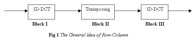
Thus the Two Dimensional formula in equation 4.1 is broken up to become two identical One Dimensional equations.

Hence, the 2D-DCT can be calculated by first calculating the 1D-DCT of the rows and then calculating the 1D-DCT of the resulting columns.

This procedure is called “The Row-Column Decomposition” algorithm. The calculation of each 1D-DCT requires (N²) additions and (N²) multiplication.

The Row decomposition requires (N2. N1²) multiplication and additions and the Column decomposition require (N1. N2²) multiplication and additions.

So to get the total 2D-DCT, it requires (N1. N2[N1+N2]) multiplication and additions. So using the Row-Column decomposition algorithm, the number of calculations are logically reduced.

For N1 = N2, the ratio of saving of calculations = (N². N²) / (2.N³) = N/2.

1. Possible Values For The Cosine Matrix

The even symmetrical formula of equation 3 can be rewritten as:

Eqn. 4

As shown, the quantity (Fi) is a function only in (n) and (k). Thus the possible numerical values for the quantity (Fi (n, k)) can be calculated separately independent on the summation forming a matrix which is called The Cosine Matrix.

These numerical values depend only on the dimensions of the output transform coefficients matrix (k1 and k2) and the dimensions of the input data matrix (N1 and N2). Starting the possible values in a cosine matrix from accessing its values when needed is considered largely a very efficient way to get the 1D-DCT because this saves large time taken during calculating the values of F (n, k).

Hence, the possible values calculated for F (n, k) are:

For the 8x8 Block 2D-DCT:

Table 5 

An important note must be declared here, The 2D-IDCT equation have the summations on 'k1' & 'k2' not 'n1' & 'n2' which can be interpreted, in matrices form, as the transposed matrix of the 2D-DCT possible values of cosine matrix.

HARDWARE IMPLEMENTATION

The hardware chosen for implementation of the DCT algorithms is the Field Programmable Gate Array (FPGA) which has widespread use in the development of Application Specific Integrated Circuits (ASICs).

The design is implemented on FPGA using Altera Max Plus II. We designed these blocks, along with the internal ones, using GDF & VHDL modules.

To improve the performance, we used the Distributed Arithmetic Algorithm.

1. Distributed Arithmetic Algorithm

The Distributed Arithmetic (DA) is an efficient procedure that targets the sum of products. In our design, each element in the input data matrix is taken 10 bits. Since each element in the input data matrix is implemented as 10 binary bits, it can be written as....

Eqn. 5

Where:

1. X_k0 = 1for negative number

= 0 for positive number

1. X_kb is the binary bit that taken a value ‘0’ or ‘1’.

1. Multiplying by (2^-b) means shifting right (b) bits.

For every row [r] in the 4x4 DCT:

Where:

1. (X_r)_kis the element (k) in row [r] in the cosine matrix.

1. (a_m)_kis the value (k) in row [m] in the cosine matrix.

By substituting with Xk from equation 3.1 we get

= - [(X_r)₁₀.(a_m)₁ + (X_r)₂₀.(a_m)₂ + (X_r)₃₀.(a_m)₃ + (X_r)₄₀.(a_m)₄]

+ [(X_r)₁₁.(a_m)₁ + (X_r)₂₁.(a_m)₂ + (X_r)₃₁.(a_m)₃ + (X_r)₄₁.(a_m)₄] 2^-1

+…

+ [(X_r)₁₉.(a_m)₁ + (X_r)₂₉.(a_m)₂ + (X_r)₃₉.(a_m)₃ + (X_r)₄₉.(a_m)₄] 2^-9

1. Design

1. 1D-DCT

This block is responsible for the bit formatting in an appropriate way to be able to address the DALUT ROM's to calculate the result of the 1D summations (1D-DCT)

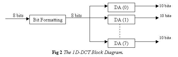
Bit Formatting Block:

10. Stores the 8-bit input values in each row.
11. Selects the 1^st Bit in each element & sends it to the DAs then selects the 2^nd Bit in each element & sends it to the DAs, & so on until the 8th value.
12. The output is completely isolated from internal operations to achieve pipelining between blocks.

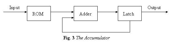
Calculation of the 1D-DCT (DA):

13. Calculates the summation for each row of the input matrix.
14. Values are input to this block one after another starting with the value representing the MSB of each Pel value.
15. Since this block is supposed to multiply numbers in Binary format which can be positive or negative (2's complement) then we need a direct method to multiply 2 Binary numbers in 2's complement format which is not available.
16. A new method were introduced to achieve the direct multiplication; it combines the signed Bit extension method & the signed numbers methods in a single approach that can be used to multiply any 2 Binary numbers in 2's complement format.
17. When multiplying 2 positive Binary numbers, we multiply each bit of the multiplicand by the multiplier; the resultant values are added after shifting them properly. To generalize it, we subtract the 1^st value & extend the sign bit of the others then add them.
18. The input values are input one after another, subtracting the 1^st value & adding the others with sign bit extension one at a time.
19. To reduce the delay, we didn't shift the values to the right but using an accumulator, we load the 2's complement of the 1^st value in it.Throw a Feed Back, the stored value in the accumulator is shifted to the left one bit (wiring) & added to the input.The concept is that shifting the result to the left one bit at a time is the same as shifting each value the right a number of bits equal to its index.
20. The output is completely isolated from internal operations to achieve pipelining between blocks.
21. A block diagram is shown below in fig 3.

1. Transposing the intermediate matrix

10. When we take a close look at the 2D-DCT equation we realize that to calculate each DCT coefficient we need the entire input matrix. The entire matrix is multiplied, Dot Product, with row (I) of the cosine matrix & again with row (J) to produce the (I, J) DCT coefficient. To save time, we multiply each row of the input matrix by the entire cosine matrix so the result will be the columns not rows of the intermediate matrix. For this reason we need to transpose this matrix.
11. It stores the column from the DAs in RAM until the matrix is completed then it output them transposed. Using 2 RAMs & a ROM (to store the sequence), we write in the 1^st in order & read from the other transposed in one period then read transposed from the 1^st & write in order in the 2^nd in another period & so on. This method was introduced to isolate the Row Decomposition from the Column Decomposition & achieve pipelining.
12. A block diagram is shown below in fig 4.

SIMULATION RESULTS

To give an overview about how the interface to our design is done and how to test our results. Both were done using a single visual basic program.

By interface we mean how to input the data to the hardware. Our input data is a matrix, each value represents the luminance value of the image pixels.

The program is divided into two parts:

1. DCT TEST:

This part takes the input data (luminance values) from a text file (datain.txt) and applies the DCT equation to obtain the DCT coefficients and output them to a file (dct.txt).

At the same time it sends this input data to the circuit to obtain the DCT coefficients.

The results from our circuit and from the software program are compared to check for errors.

2. IDCT TEST:

This part takes DCT coefficients from dct.txt file, applies the IDCT equation to obtain IDCT coefficients and stores them into idct.txt file. At the same time it sends these DCT coefficients to the circuit to obtain the IDCT coefficients. The results from our circuit and from the software program are compared to check for errors.

N.B:

To send any data to our circuit, it is converted to binary format then sent to the parallel port element by element. From the 10 bits, we send the least significant 8 bits to the port 378 (active high), and the most significant 2 bits are sent to the port 37A (active low). After each element (10 bits) is sent to the parallel port, we send a “1” then a “0” on the most significant bit of port 37A to announce that there is an element ready on the port (this is applied to “Data_Ready” input pin of chip).

Another program were made, using C language, which takes a picture, divided into Pixels each of which has given 8 Bits to represent its luminance value. We used this program to decide how many digits are enough for the cosine values since we are going to store there possible combinations in ROM's. The decision was based on performing the 2D-DCT then the 2D-IDCT then transform the luminance values back into Pixel level to reconstruct the image again.

The decision was based on performing the 2D-DCT then the 2D-IDCT then transform the luminance values back into Pixel level to reconstruct the image again.

As an example for the 8x8 2D-DCT design, we represent an input matrix, ideal DCT matrix and the actual DCT matrix from our design:

Input matrix of Luminance values of Pels.

Actual DCT coefficients.

Output matrix of DCT coefficients.

To reduce Hardware needed for the previous design, we used a different algorithm. This algorithm by Chen et al uses the symmetry in the cosine matrix to implement the 8x8 1D-DCT / IDCT using two 4x4 1D-DCT / IDCT which reduces gradually the Hardware & increase the maximum speed.

The cosine matrix for the 2D-DCT can be written as shown:

The symmetry in this matrix can be exploited and the 1D-DCT will then be rearranged to give:

y₀      = D D D D       *        x₀ + x₇

y₂                B F -F -B                   x₁ + x₆

y₄                  D -D -D D                   x₂ + x₅

y₆                  F -B B -F                   x₃ + x₄

AND

y₁      = A C E G        * x₀ - x₇

y₃                 C -G -A -E                  x₁ - x₆

y₅                  E -A G C                  x₂ - x₅

y₇                 G -E C -A                  x₃ - x₄

The (N x N) multiplication matrix has been replaced by two (N/2) x (N/2) matrices, which can be computed in parallel as can the sums and differences forming the vectors on the right hand side. The implementation requires 32 multiplication instead of 64 multiplication.

To implement the 1D-IDCT, we must use the transposed cosine matrix, which leads to another rearrangement:

Adding (y₀ + y₇) and (y₀ - y₇) we obtain y₀ and subtracting them we obtain y₇ and so on for the rest of the 1D-IDCT outputs.

From the previous equation, we can realize that it's the second matrix is the same as in the 1D-DCT since it's a symmetrical matrix. Also, the Hardware implementation for the 1D-IDCT will be simpler since the summation and subtraction are done for the output and not the input as in the 2D-DCT.

An important advantage arises in this design, the maximum allowable speed will increase up to 111.11 MBit/sec since we are using the 4x4 DA multiplication knowing that both parts must work in parallel to save time. This requires dividing the Master Clock signal by two for the 4x4 DA multiplication to compute correctly.

As an example for the 8x8 2D-DCT design, we represent an input matrix, ideal DCT matrix and the actual DCT matrix from our design:

Input matrix of DCT coefficients.

Actual Luminance values of Pels.

Output matrix of Luminance values of Pels.

The average error, between the exact values and the output values from the simulation results, can be found as less than 1.2%

We have made complete design of the 8x8 2D-DCT and 8x8 2D-IDCT designs with 10 input bits for IDCT and 8 input bits for DCT with bit duration of at least 18 nsec, which is equivalent to a max bit rate of 55.55Mbits/sec.

We were unable to put the memory of the DCT & IDCT of the 8x8 Block in a single Altera FPGA chip since the size is. However, this size is reduced due to the symmetry in the cosine matrix, since the cosine is a periodic function.

The Chen et al algorithm (2) helped us reduce the memory size since it transforms the 8x8 1D-DCT / IDCT into two 4x4 1D-DCT / IDCT and increases the speed into 111.11Mbit/sec.

We are currently investigating reducing the number of bit per word to reduce the losses in the memory utilization to use the hardware more efficiently. This has major impact on the memory size needed to use a smaller chip (Altera Flex 10KE EPF10k100). 

1. MPEG Video Compression Standard
2. G.S. Taylor & G.H. Blair “Design for the Discrete Cosine Transform in VLSI “ (IEEE 1998).
3. Les Mintzer. “The rule of Distributed Arithmetic in FPGA-Based signal processing”
4. Helal Ibrahim Helal , Ali Ezzat , Samia Mashali “Realization of FPGA-Based 2D-DCT “
5. Sean Keating (Dublin City Univ.) “Toword Hardware implementation of 2D-DCT Image Processing Algorithm”
6. V.Srini Vasan & K.J.R.Liu “VLSI Design of High-Speed time recursive 2D-DCT / IDCT processor for video application”.
7. David Pellirin & Douglas Taylor “VHDL made easy “.
8. Digital Computer Design Fundamentals
9. M. Sanchez, J. Bolgera & E. L. Zabata “Bit-Serial Architecture for the 2D-DCT”.
10. www.altera.com

Package used: Altera Max Plus ll.

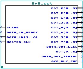
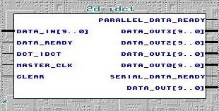
... 4x4 Block Chip Description ...